Tensor network diagrams of typical neural networks
The starting point of all neural network is the “neuron”, i.e. the following operation on input $\vec x$:
\begin{align}
h_{i}=g\left(\sum_{j}W_{ij}x_{j}+b_{i}\right)
\label{oneLayer}
\end{align}
where $\vec h$ is the ouput vector of the layer, $\vec W$ is the matrix of weights, $\vec b$ is the vector of offsets, and $g(z)$ is the activation function (typically a ReLU gate, sigmoid function, a tanh function, etc.).
For $l$ layers, the final output of the network would be the output of the last layer $\vec y=\vec h^{(l)}$.
In the the Deep Learning book, the above equation is pictured as:
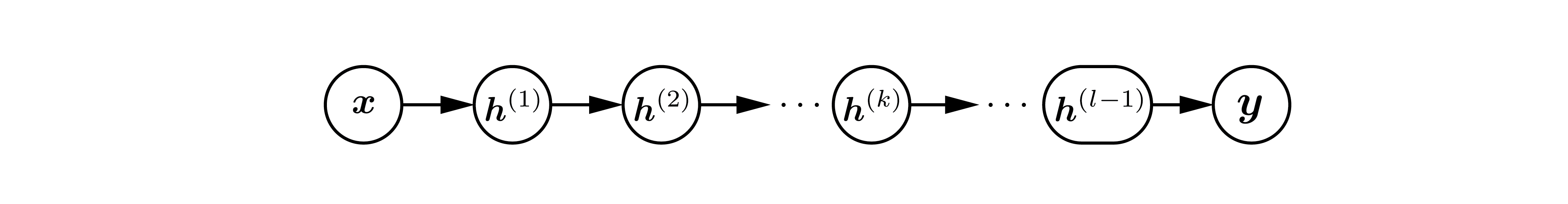
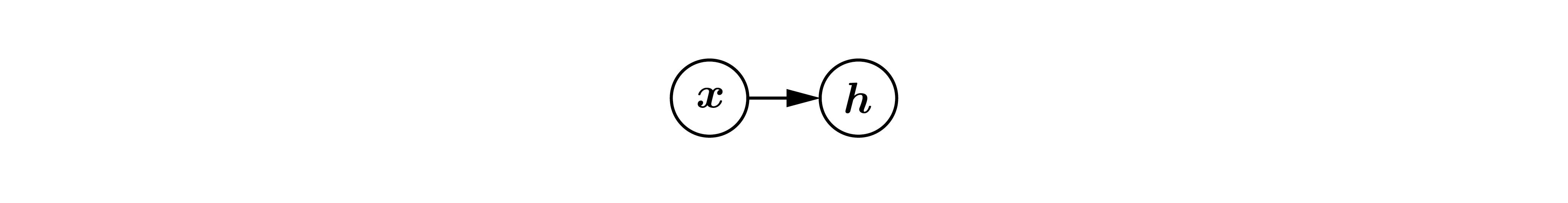 with the weights, offsets, and activation function implicit. Within this diagrammatic convention, here is what a fully connected $l$ layers neural network, or “multi-layer perceptron” (MLP), looks like:
Problems of these diagrams
At first, I did not like this diagrammatic convention. I thought you need to know the equations represented to be able to understand the diagrams. A good example is when the reccurent neural network (RNN) is introduced:
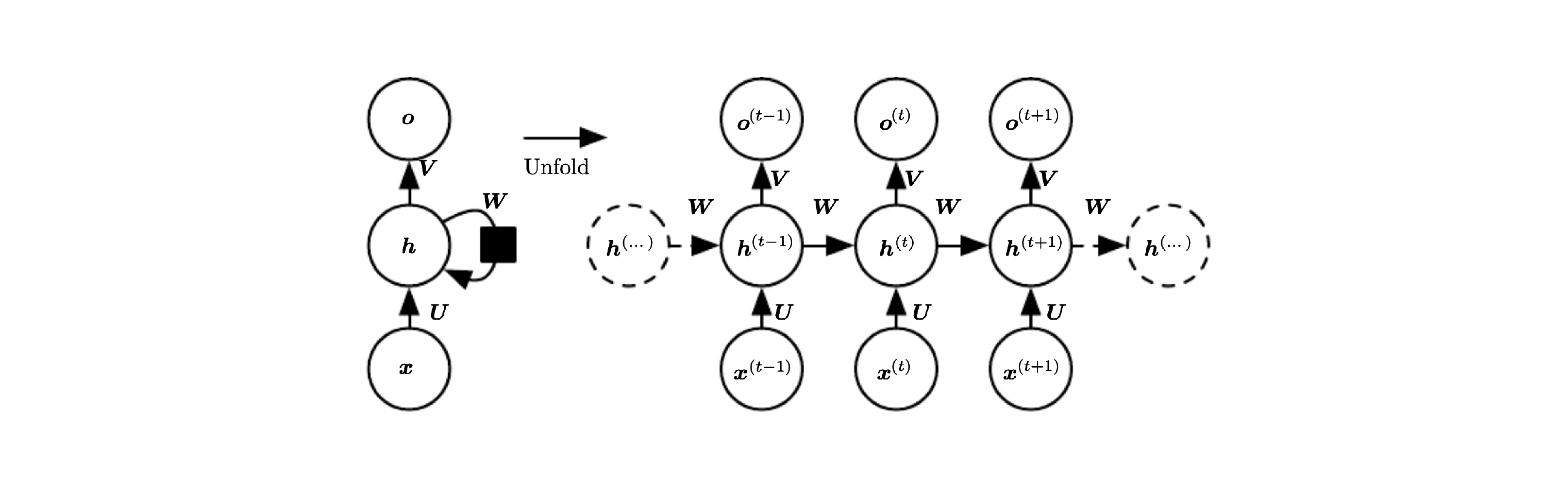 The reader might understand that $\vec U$ and $\vec W$ are weights applied respectively on the input $x^{(t)}$ recieved at time $t$ and hidden state $h^{(t-1)}$ computed at time $t-1$, but what happens exactly to the results of these two? are they added, multiplied or concatenated to form $h^{(t)}$? Are they separately passed into a non-linear gate? Although the picture makes it unclear, the equations:
\begin{align}
\vec a^{(t)} &= \vec b + \vec W\vec h^{(t-1)} + \vec U\vec x^{(t)}
\\
The reader might understand that $\vec U$ and $\vec W$ are weights applied respectively on the input $x^{(t)}$ recieved at time $t$ and hidden state $h^{(t-1)}$ computed at time $t-1$, but what happens exactly to the results of these two? are they added, multiplied or concatenated to form $h^{(t)}$? Are they separately passed into a non-linear gate? Although the picture makes it unclear, the equations:
\begin{align}
\vec a^{(t)} &= \vec b + \vec W\vec h^{(t-1)} + \vec U\vec x^{(t)}
\\
\vec h^{(t)} &= \tanh(\vec a^{(t)})
\\
\vec o^{(t)} &= \vec c + \vec V\vec h^{(t)}
\end{align}
not only answers that they are added (although you can show concatenating yields to the same thing), and then the result is passed to the non-linear gate, we now also know it is a tanh gate. Moreover, two offsets $\vec b$ are unnecessary in this context; only one is needed. In short, the diagrammatic notation cannot be directly translated to the maths. I consider this a big prolem compared, for example, to Feynman diagrams, which became famous and widely used mainly because they translate directly to equations.
Tensor network notation in physics
In the winter of 2018, I followed a course on tensor network methods for strongly correlated electrons given by Glen Evenbly at Université de Sherbrooke. Basically, the course introduces a diagrammatic notation to write tensor products, and uses it to revisit famous methods of strongly correlated physics, among which the numerical renormalization group (NRG), density matrix renormalization group (DMRG), matrix product states (MPS), multi-scale entanglement renormalization ansatz (MERA), etc.
Here are the basics: vector have one leg (because they have one index), matrix have two, and more general tensors have as many as their order. You can then illustrate a tensor product by connecting the legs corresponding to the index summed.
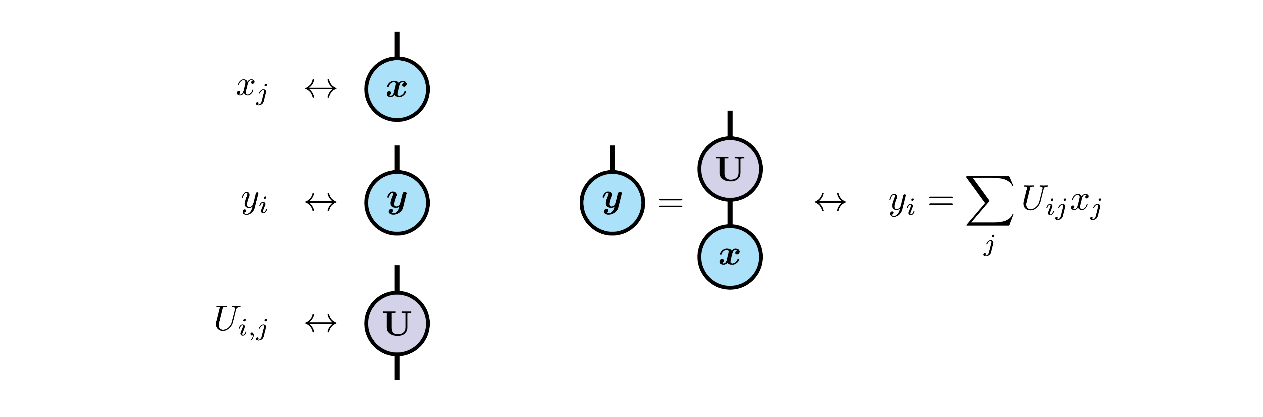
Since I began working on neural networks, I tried to draw the tensor network diagram corresponding to a few architecture visited in the DL book. Trying to clean the diagrammatic representation of all ambiguity helped me understand many things. For example, here is the representation of a simple hidden unit using a sigmoid gate $\sigma(z)$:
\begin{align}
h_{i}=\sigma\left(\sum_{j}W_{ij}x_{j}+b_{i}\right)
\end{align}
 Here is how the deep neural network illustrated at the beginning would look like:
 with $g^{(k)}$ telling what non-linear gate is used at each layer. Note that I augmented the notation with element-wise operations, illustrated as teardrops (with their corner indicating the ouput of the operation), and with the non-linear functions, illustrated as arrowheads.
Disclaimer
There is one fundamental difference between the tensor network notation used in physics and the graphical notation used for neural networks. In physics, combining different quantum systems correspond to a tensor product. Because of this, two parallel legs in tensor networks correspond to building the tensor product space of those two dimension.
 With neural networks, however, the dimension of such tensor product would grow too fast to be practical, and parallel lines (and, often, merging lines) denote a direct sum (a concatenation).
 Because of this, the diagrams I show below are more an exercise to understand neural networks rather than accepted tensor network diagrams of neural networks. This is also why I needed an explicit notation for addition (concatenation) of vectors, which is not standard in tensor network diagrams.
Tensor network notation for (RNN)
Here is a RNN’s hidden unit, following the DL book’s equations 10.8-10.9 (same as above), but here unified in a single index notation equation:
\begin{align} h^{(t)}_i &=\tanh\left(b_{i}+\sum_{j}W^{\phantom t}_{i,j}h_{j}^{(t-1)}+\sum_{j}U^{\phantom t}_{i,j}x_{j}^{(t)}\right) \end{align}
 while the full RNN (with the previous diagram explicitely appearing for $h_{j}^{(t)}$), looks like:
\begin{align} y_{i}^{(t)}&=\operatorname{softmax}\left(c_{i}+\sum_{j}V_{i,j}h_{j}^{(t)}\right) \end{align}
 In the above diagram, the loop means that the intermediate output $\vec h$ at time $t-1$ is used as an extra input at time $t$. One can see this more clearly by unfolding the network, as usually done with RNNs:

Long short-term memory (LSTM)
I do not explain the LSTM unit here, since the introduction by Chris Colah is excellent, and well known. However, I still find his illustration a little bit ambiguous, so here is the corresponding tensor network I came up with. Here, I follow the DL book’s equations 10.40-10.44.
The first step is to draw the internal state, as it is the most complicated diagram (where $\odot$ are element-wise products):
\begin{align}
s_{i}^{(t)}=f_{i}^{(t)}s_{i}^{(t-1)}+g_{i}^{(t)}\sigma\bigg(b_{i}+\sum_{j}U_{i,j}x_{j}^{(t)}+\sum_{j}W_{i,j}h_{j}^{(t-1)}\bigg)
\end{align}
 Then we notice that $\vec f$ and $\vec g$ and $\vec q$ (the latter do not appear explicitely above, but it is necessary to get $\vec h$ below) are all equivalent units with different parameters:
\begin{align}
f_{i}^{(t)}=\sigma\bigg(b_{i}^{f}+\sum_{j}U_{i,j}^{f}x_{j}^{(t)}+\sum_{j}W_{i,j}^{f}h_{j}^{(t-1)}\bigg)\end{align}
\begin{align}
g_{i}^{(t)}=\sigma\bigg(b_{i}^{g}+\sum_{j}U_{i,j}^{g}x_{j}^{(t)}+\sum_{j}W_{i,j}^{g}h_{j}^{(t-1)}\bigg)
\end{align}
\begin{align}
q_{i}^{(t)}=\sigma\bigg(b_{i}^{o}+\sum_{j}U_{i,j}^{o}x_{j}^{(t)}+\sum_{j}W_{i,j}^{o}h_{j}^{(t-1)}\bigg)
\end{align}
\begin{align}
h_{i}^{(t)}=\tanh\big(s_{i}^{(t)}\big)q_{i}^{(t)}
\end{align}
Therefore, in the end, the complete LSTM diagram looks like this:
Then we notice that $\vec f$ and $\vec g$ and $\vec q$ (the latter do not appear explicitely above, but it is necessary to get $\vec h$ below) are all equivalent units with different parameters:
\begin{align}
f_{i}^{(t)}=\sigma\bigg(b_{i}^{f}+\sum_{j}U_{i,j}^{f}x_{j}^{(t)}+\sum_{j}W_{i,j}^{f}h_{j}^{(t-1)}\bigg)\end{align}
\begin{align}
g_{i}^{(t)}=\sigma\bigg(b_{i}^{g}+\sum_{j}U_{i,j}^{g}x_{j}^{(t)}+\sum_{j}W_{i,j}^{g}h_{j}^{(t-1)}\bigg)
\end{align}
\begin{align}
q_{i}^{(t)}=\sigma\bigg(b_{i}^{o}+\sum_{j}U_{i,j}^{o}x_{j}^{(t)}+\sum_{j}W_{i,j}^{o}h_{j}^{(t-1)}\bigg)
\end{align}
\begin{align}
h_{i}^{(t)}=\tanh\big(s_{i}^{(t)}\big)q_{i}^{(t)}
\end{align}
Therefore, in the end, the complete LSTM diagram looks like this:
 Can you find on what branches $\vec f$, $\vec g$ and $\vec q$ are now respectively found?