Dispersion of cuprates

When working on high temperature superconducting cuprates, there is one simple model everybody starts from. It is often surprising how much this model captures, and so it is important to compare more sophisticated theories, for example those taking into account strong correlations, to this simple non-interacting model. This post describes this single-band non-interacting model of cuprates.

Two-dimensional dispersion

Since cuprates are highly bidimensional, a 2D model is often enough. The non-interacting starting point in 2D for any cuprates is the following energy function:

$$\begin{align} \epsilon_{\vec k} &= -2t\big(\cos (k_xa) + \cos (k_yb)\big) \nonumber\\\ &\phantom{=\ } -4t'\cos (k_xa)\cos (k_yb) \nonumber\\\ &\phantom{=\ } -2t''\big(\cos (2k_xa)+\cos (2k_yb)\big) \end{align}$$

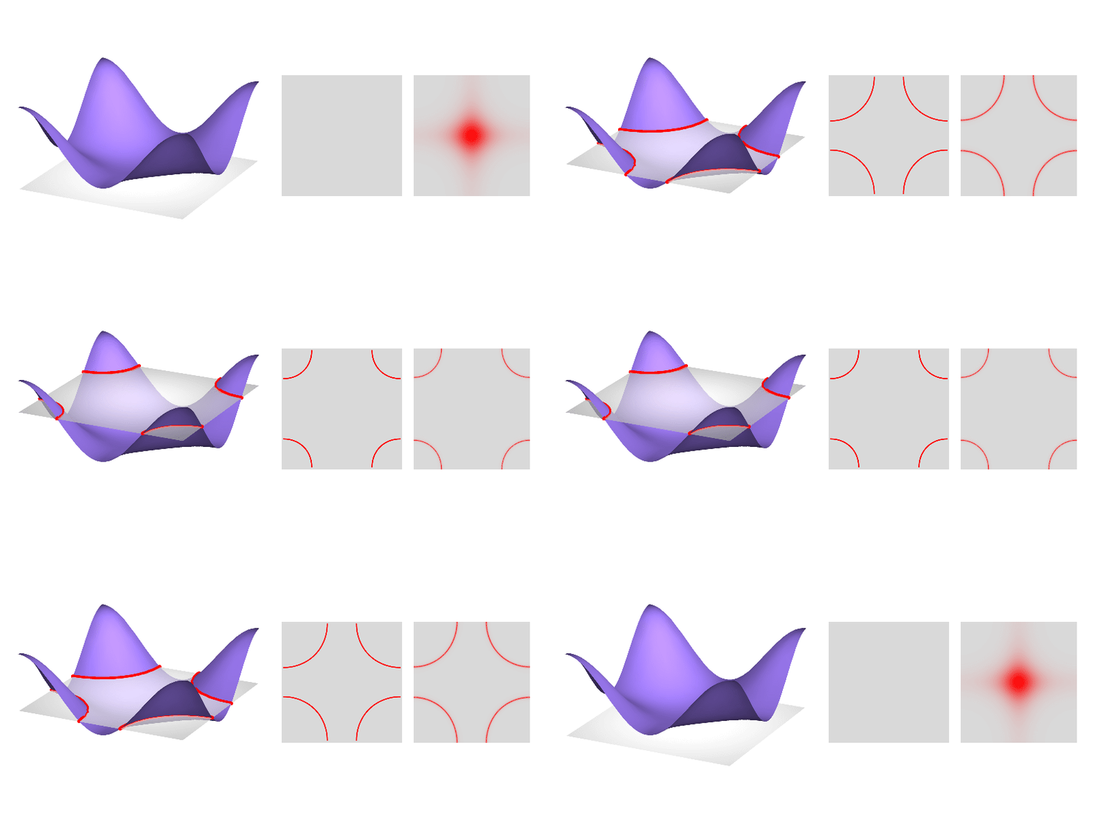
where $t$, $t’$, and $t’’$ are the first, second and third neighbour hopping, respctively. The chemical potential $\mu$ can be added as $\xi_{\vec k}=\epsilon_{\vec k}-\mu$. A simplified, and typical dispersion can be obtained with $t=1$, $t’=-0.35$, and $t’‘=0$. Of course, such a simple model does not contain superconductivity. As a function of $k_x$ and $k_y$, this energy function can be visualize as below. In this animation, the left plot shows $\xi_{(k_x,k_y)}=\epsilon_{(k_x,k_y)}-\mu$ as a function of $k_x$ and $k_y$, with the chemical potential $\mu$ changing in time. In the center, I plot the energy contour $\xi_{(k_x,k_y)} = 0$ as a function of $k_x$ and $k_y$, and on the right, the spectral weight at the Fermi level $A(\vec k, \epsilon=0)$. The latter is the same as the energy contour in this case, and it is computed with:

$$\begin{align} A(\vec k, \epsilon) = -\frac{1}{\pi}\text{Im}\left\{\frac{1}{\epsilon+i0^{+}-\xi(\vec k)}\right\} \end{align}$$

where $0^+$ takes an arbitrary small value, (in this case 0.05). More information on the spectral weight is given in my visual introduction to Green’s function. The Mathemtatica code to produce the above animation is given below.

Three dimensional dispersion

Real cuprates are 3D materials. The extension of the above model to the three-dimensional dispersion is given by (see Horio 2018 for ARPES measurement, and Markiewicz 2005 for theoretical justifications):

$$\begin{align} \epsilon_{\text{3D}}(\vec k)=\epsilon_{\vec k}+\epsilon_{\perp}(\vec k) \end{align}$$ where $\epsilon_{\vec k}$ is the same as above and $\epsilon_{\perp}(\vec k)$ is the inter-plane dispersion:

$$\begin{align} \epsilon_{\perp}(\vec k) &= -2t_z\cos(k_xa/2) \cos(k_yb/2) \cos(k_zc/2) (\cos (k_xa) - \cos (k_yb))^2. \end{align}$$

The experimental fit by Horio 2018 in Eu-LSCO yields parameters $a=b=3.75$, $c=13.20$, $t=190$ meV, $t’=-0.14t$, $t’‘=0.07t$, and $t_z0.07t$.

Doping

The chemical potential $\mu$ is obtained by solving the integral equation for a given doping $p$:

$$\begin{align} p &= 1 - n \\ &= 1 - \iiint_{BZ} \frac{d^{3}k}{4\pi^{3}} f(\epsilon_{\text{3D}}(\vec k)-\mu) \end{align}$$ One can put $t_z=0$ to get the 2D case.

Approximation for the pseudogap

To fit the results for the pseudogap regime at $p\lt p^*$, we need some way to simulate the mysterious pseudogap ``phase’’, which is an active area of research. One way that seems to work fairly well is to start from a two-dimensional antiferromagnetic (AF) reconstruction of the bare band (following recent success of such a model for the Hall number by Storey 2016 (We published a follow-up paper on this):

$$\begin{align} E^{\pm}(\vec k) = \tfrac{1}{2}(\epsilon_{\vec k}+\epsilon_{\vec k+\vec Q}) \pm \sqrt{ \tfrac{1}{4}(\epsilon_{\vec k}-\epsilon_{\vec k+\vec Q})^2 + M^2} \end{align}$$ We cannot extend this model straightforwardly to the three-dimensional dispersion, because taking $\epsilon_{\vec k}\rightarrow\epsilon_{\text{3D}}(\vec k)$ in the above equation results in C4 rotational symmetry breaking. This is because of the body-centered structure of Nd-LSCO, which is fully taken into account in $\epsilon_\perp(\vec k)$, and in for which antiferromagnetism is not the same for $\vec Q=(\pi/a,\pi/a,0)$ than for $\vec Q=(\pi/a,-\pi/a,0)$. What somewhat works, instead, is to suppose that the 2D planes contain independent antiferromagnetic orders, and add the $z$-dispersion after the reconstruction:

$$\begin{align} E^{\pm}_{\text{3D}}(\vec k)=E^{\pm}(\vec k)+\epsilon_{\perp}(\vec k) \end{align}$$

This may be interpreted as antiferromagnetism uncorrelated between planes.

Mathematica code for the animation

xi[kx_, ky_] = -2*(Cos[kx] + Cos[ky]) + 
   2*0.35*(Cos[kx + ky] + Cos[kx - ky]);
spectralWeight[kx_, ky_, w_, mu_] := 
  0.05/((w - xi[kx, ky] + mu)^2 + 0.05^2)/Pi;

spWeightColor[x_] := 
  Blend[{{0, LightGray}, {1, RGBColor[1, 0, 0, 1]}}, x];
SetOptions[Plot3D, Mesh -> None, Boxed -> False, Ticks -> None, 
  Axes -> False, PlotRange -> Full, BoxRatios -> {1, 1, 0.6}, 
  BoundaryStyle -> None, MaxRecursion -> 7, ClippingStyle -> None, 
  Ticks -> None, 
  Lighting -> {{"Point", White, {0, 0, 12}}, {"Point", 
     White, {-20, -20, 0}}}, ViewPoint -> {-10, -5, 4}];
SetOptions[ContourPlot, FrameTicks -> None, Frame -> None, 
  AspectRatio -> 1];
SetOptions[DensityPlot, FrameTicks -> None, PlotPoints -> 70, 
  Frame -> None, AspectRatio -> 1, ColorFunction -> spWeightColor];

x = 0.16;
T = Table[
   GraphicsRow[{
     Plot3D[{xi[kx, ky], mu - 0.03}, {kx, -Pi, Pi}, {ky, -Pi, Pi}, 
      PlotRange -> {-4, 6}, 
      PlotStyle -> {{RGBColor[0.45, 0.35, 0.7, 1], 
         Opacity[1]}, {White, Opacity[0.7]}, {White, Opacity[0.8]}}, 
      MeshStyle -> Directive[Thickness -> 0.01, Red], 
      MeshFunctions -> {#3 &}, Mesh -> {{mu}}
      ],
     GraphicsRow[{
       ContourPlot[{xi[kx, ky] == mu}, {kx, -Pi, Pi}, {ky, -Pi, Pi}, 
        ContourStyle -> {Thickness -> 0.01, Red}, 
        Prolog -> {LightGray, 
          Rectangle[Scaled[{0, 0}], Scaled[{1, 1}]]}
        ],
       DensityPlot[
        spectralWeight[kx, ky, 0, mu], {kx, -Pi, Pi}, {ky, -Pi, Pi}, 
        PlotRange -> {0, 10}]
       }]
     }, ImageSize -> Full, Background -> White]
   , {mu, Range[-300, 350, 50]/100.0 + 0.01}];

Export["CupratesMovie.gif", Join[T, Reverse[T]], 
 "AnimationRepetitions" -> Infinity]